Amplitude estimation is a sophisticated algorithm that outperforms standard Monte Carlo (MC) approaches by a factor of four. It has a variety of applications, including quantum chemistry, machine learning, and finance, where it can aid in risk analysis and financial derivatives trading. In a study in the journal Quantum, researchers consider whether quantum algorithms can reduce the quantum computational needs for amplitude estimation further.
Study: Variational quantum amplitude estimation. Image Credit: vs148/Shutterstock.com
The original amplitude estimation approach includes hardware requirements that are difficult to meet with today’s quantum devices; therefore, lowering these needs is a hot topic of research right now. Recent suggestions that succeeded in substituting the hardware-intensive components of conventional amplitude estimation—controlled multi-qubit gates and quantum Fourier transform—with classical post-processing achieved crucial advancements.
Furthermore, by interpolating between classical MC approaches and amplitude estimation, the circuit depth can be systematically reduced. Moreover, in the presence of device faults, classical pre-processing can be utilized to substitute expensive quantum arithmetic, and Bayesian inference can be employed to improve algorithmic efficiency.
Researchers offer variational quantum amplitude estimation (VQAE), which uses variational optimization to keep the depth of the complete quantum circuit below a specified maximum value. Maximum likelihood amplitude estimation (MLAE) underpins VQAE.
Figure 1 shows that VQAE outperforms classical MC sampling for the problems considered here, while also keeping the overall circuit depth below a given value.
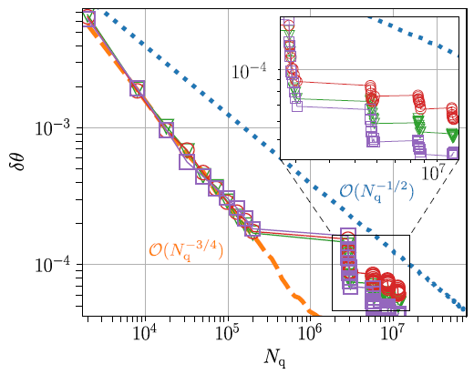
Figure 1. Amplitude estimation error δθ as a function of the computational cost, i.e. the number of queries Nq. We compare adaptive VQAE (symbols with lines guide to the eye) to MLAE (dashed orange) and classical MC sampling (dotted blue). We calculate the rescaled mean value of a shifted Cauchy-Lorentz (red circles), Gaussian (green triangles), and log-normal (purple squares) probability distribution. In VQAE, the first 10 amplitude estimates are computed via MLAE, then one step of the variational optimization is performed, which is followed by the next iteration of 10 MLAE steps. This procedure of variational approximation followed by MLAE is repeated three more times, resulting in a final error δθ ≈ 6 · 10−5. We see that, for this error, Nq is up to an order of magnitude smaller in VQAE than in classical MC sampling. Throughout this calculation, VQAE’s circuit depth is the depth of the initial state plus at most 10 times the depth of the query operator, whereas MLAE’s circuits have the depth of the initial state plus, at the end, 50 times the depth of the query operator. Image Credit: Plekhanov, et al., 2022
Discussion
Researchers begin by defining the problem that they are interested in this part. Following this, researchers explain quantum amplitude estimation and classical MC sampling in detail. Researchers look at three different probabilities: Gaussian, Cauchy-Lorentz, and log-normal distribution.
Various recent publications propose new approaches to carry out amplitude estimation without using quantum phase estimation or deep quantum circuits to avoid deep quantum circuits.
The variational algorithms are presented in this study. The general VQAE concept is first explained, followed by the naive implementation, and finally, the adaptive VQAE technique.
The VQAE algorithm is based on a linearly incremental sequence and a maximum likelihood framework. Researchers add a variational step to this framework to avoid the circuit depth from expanding endlessly.
The variational approach, on the other hand, allows computing the approximation error and determining when the strategy is effective (Figure 2).

Figure 2. Variational PQC ansatz of depth d for 6 qubits. The variational parameters λj are in single-qubit rotation gates Ry(λj ) = exp(−iλjσy/2) where σy denotes the y Pauli matrix. In naïve VQAE, |φinit⟩n+1 = |0⟩n+1 and the circuit structure inside the dashed box is repeated d times. In adaptive VQAE, |φinit⟩n+1 = |χ0⟩n+1 and only the dark blue gates with adjacent CNOTs form our variational ansatz. Image Credit: Plekhanov, et al., 2022
The gradient-based technique combined with the Adam optimizer yielded the greatest results. As a result, this method will be utilized to compute all of the results in this article.
The number of inquiries required per variational approximation is considered to be independent of the iteration number m and only varies as a function of the desired variational error and the depth of the circuit for the objective function.
When the MLAE error is smaller than the variational error, the latter dominates the convergence. A randomized procedure can be used to simulate the buildup of variational error, in which each variational approximation results in a random error with a zero mean and some variance (Figures 3 and 4).
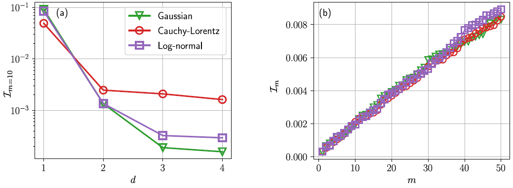
Figure 3. Infidelity Im in Eq. (22) for the probability distributions of Eqs. (2)-(4) (see legend) shown (a) as a function of d for m = 10 and (b) as a function of m for d = 4. We see that the infidelity decreases with increasing d, due to the corresponding increase of the expressive power of the PQC. The infidelity increases linearly as a function of m slowly with a slope of ≈ 0.00017 that is approximately the same for the three distributions. These results are obtained via naïve VQAE with k = 1, M = 50, and ns = 1000, using the numerically exact gradient without sampling and Adam with the initial learning rate β = 0.1. We consider 100 randomly initialized PQC and (a) shows one example calculation and (b) the average over all 100 calculations. Image Credit: Plekhanov, et al., 2022
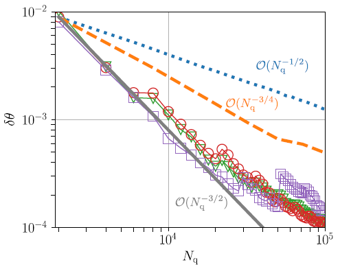
Figure 4. Amplitude estimation error δθ as a function of the number of queries Nq obtained using naïve VQAE with k = 1 under the assumption of zero variational cost Nvar/1 = 0. We observe that for small M, the error follows the ideal VQAE scaling δθ ∼  (Nq−3/2) (solid gray line). For larger values of M, the scaling changes to the MC scaling δθ ∼
  (Nq−1/2) (dotted blue line). The result is also compared to the MLAE scaling δθ ∼
  (Nq−3/4) (dashed orange line). The legend as well as the simulation parameters is the same as in Figure 3. Image Credit: Plekhanov, et al., 2022
Finally, researchers consider the cost of the variational approximation to get a better complete picture of every VQAE’s algorithmic efficiency.
Figure 2 shows the performance of the adaptive VQAE algorithm using a simpler variational ansatz consisting of only six single-qubit rotation gates and four CNOT gates. The amount of variational queries, as well as the impacts of noise due to finite sampling, is greatly reduced with this simpler approach, which has just six parameters in total.
Researchers ran the same simulations as in Figure 1 for n = 8, 10, and 12 to see how adaptive VQAE performs when qubit counts n increase. Figure 5 shows the findings for the Gaussian probability distribution. Researchers achieved results that were on top of the ones in Figure 5 for the shifted Cauchy-Lorentz and log-normal probability distributions.
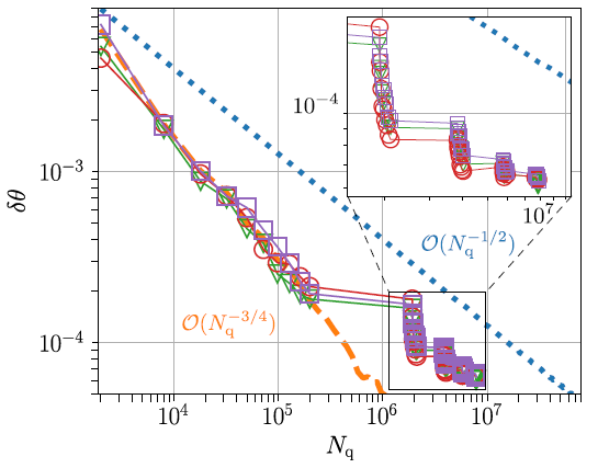
Figure 5. Amplitude estimation error δθ as a function of the number of queries Nq for adaptive VQAE with n = 8 (green triangles), 10 (red circles), and 12 (purple squares) qubits for the Gaussian probability distribution in Eq. (2). The remainder of the legend and the optimization procedure are the same as in Figure 1. Image Credit: Plekhanov, et al., 2022
Conclusion
In this paper, researchers show that in the setting of amplitude estimation, variational quantum algorithms based on constant depth quantum circuits can be more effective than classical MC sampling. However, the quantum circuits used in the numerical simulations are still difficult to implement in this generation of gate-based quantum computers.
As a result, finding new problems and applications for which VQAE has low quantum hardware needs and can be achieved on genuine quantum devices is a fascinating next step.
VQAE could be used in a variety of fields in the future, including combinatorial optimization, quantum machine learning, and quantum chemistry.
It is also intriguing to see if a variational Grover search algorithm can gain from filtering operators in this case.
Researchers believe that the VQAE algorithm’s efficiency can be improved further. It would be great to see whether there are any other ways that perform better.
Journal Reference:
Plekhanov, K., Rosenkranz, M., Fiorentini, M., Lubasch, M. (2022) Variational quantum amplitude estimation. Quantum, 6, p. 670. Available Online: https://quantum-journal.org/papers/q-2022-03-17-670/pdf/
References and Further Reading
- Brassard, G., et al. (2002) Quantum amplitude amplification and estimation. AMS Contemporary Mathematics, 305, pp. 53–74. doi.org/10.48550/arXiv.quant-ph/0005055.
- Montanaro, A (2015) Quantum speedup of Monte Carlo methods. Proceedings of the Royal Society A: Mathematical, Physical and Engineering Sciences, 471(2181). doi.org/10.1098/rspa.2015.0301.
- Knill, E., et al. (2007) Optimal quantum measurements of expectation values of observables. Physical Review A, 75(1) p. 012328. doi.org/10.1103/PhysRevA.75.012328.
- Kassal, I., et al. (2008) Polynomial-time quantum algorithm for the simulation of chemical dynamics. Processing of the National Academy of Sciences of the USA, 105(48), pp. 8681–18686. doi.org/10.1073/pnas.0808245105.
- Wiebe, N., et al. (2015) Quantum Algorithms for Nearest-Neighbor Methods for Supervised and Unsupervised Learning. Quantum Information & Computation, 15(3-4), pp. 316–356. doi/10.5555/2871393.2871400.
- Wiebe, N., et al. (2016) Quantum Deep Learning. Quantum Information & Computation, 16(7-8), pp. 541–587. doi/10.5555/3179466.3179467.
- Kerenidis, I., et al. (2019) qmeans: A quantum algorithm for unsupervised machine learning. Advances in Neural Information Processing Systems, 32. doi.org/10.48550/arXiv.1812.03584.
- Orús, R., et al. (2019) Quantum computing for finance: Overview and prospects. Reviews in Physics, 4, p. 100028. doi.org/10.1016/j.revip.2019.100028.
- Egger, D. J., et al. (2020) Quantum Computing for Finance: State-of-the-Art and Future Prospects. IEEE Transactions on Quantum Engineering, 1, pp. 1–24. doi.org/10.1109/TQE.2020.3030314.
- Bouland, A., et al. (2020) Prospects and challenges of quantum finance. Quantum Physics (quant-ph). doi.org/10.48550/arXiv.2011.06492.
- Woerner, S & Egger, D J (2019) Quantum risk analysis. npj Quantum Information, 5, p15. doi.org/10.1038/s41534-019-0130-6.
- Braun, M. C., et al. (2021) A Quantum Algorithm for the Sensitivity Analysis of Business Risks. Quantum Physics (quant-ph). doi.org/10.48550/arXiv.2103.05475.
- Rebentrost, P., et al. (2018) Quantum computational finance: Monte Carlo pricing of financial derivatives. Physical Review A, 98, p. 022321. doi.org/10.1103/PhysRevA.98.022321.
- Stamatopoulos, N., et al. (2020) Option Pricing using Quantum Computers. Quantum, 4, p. 291. doi.org/10.22331/q-2020-07-06-291.
- Suzuki, Y., et al. (2020) Amplitude estimation without phase estimation. Quantum Information Processing, 19, p. 75. doi.org/10.1007/s11128-019-2565-2.
- Tanaka, T., et al. (2021) Amplitude estimation via maximum likelihood on noisy quantum computer. Quantum Information Processing, 20, p. 293. doi.org/10.1007/s11128-021-03215-9.
- Aaronson, S & Rall, P (2020) Quantum approximate counting, simplified. In: Symposium on Simplicity in Algorithms, SIAM, pp. 24–32. doi.org/10.1137/1.9781611976014.5.
- Grinko, D., et al. (2021) Iterative quantum amplitude estimation. Npj: Quantum Information, 7, p. 52. doi.org/10.1038/s41534-021-00379-1.
- Giurgica-Tiron, T., et al. (2020) Low depth algorithms for quantum amplitude estimation. Quantum Physics (quant-ph). doi.org/10.48550/arXiv.2012.03348.
- Herbert, S (2021) Quantum Monte-Carlo Integration: The Full Advantage in Minimal Circuit Depth. Quantum Physics (quant-ph), p. arXiv:2105.09100. doi.org/10.48550/arXiv.2105.09100.
- Wang, G., et al. (2021) Minimizing Estimation Runtime on Noisy Quantum Computers. PRX Quantum, 2, p. 010346. doi.org/10.1103/PRXQuantum.2.010346.
- Katabarwa, A., et al. (2021) Reducing runtime and error in VQE using deeper and noisier quantum circuits. Quantum Physics (quant-ph), p. arXiv:2110.10664. doi.org/10.48550/arXiv.2110.10664.
- Benedetti, M., et al. (2019) Parameterized quantum circuits as machine learning models. Quantum Science and Technology, 4(4), p. 043001. doi.org/10.1088/2058-9565/ab4eb5.
- Cerezo, M., et al. (2021) Variational quantum algorithms. Nature Reviews Physics, 3, pp. 625–644. doi.org/10.1038/s42254-021-00348-9.
- Bharti, K., et al. (2022) Noisy intermediate scale quantum algorithms. Reviews of Modern Physics, 94(1), p. 015004. doi.org/10.1103/RevModPhys.94.015004.
- Brassard, G & Hoyer P (1997) An exact quantum polynomial-time algorithm for Simon’s problem. In Proceedings of the Fifth Israeli Symposium on Theory of Computing and Systems, pp 12 to 23. IEEE. doi.org/10.1109/ISTCS.1997.595153.
- Grover, L. K (1998) Quantum computers can search rapidly by using almost any transformation. Physical Review Letters, 80 (19), p.4329. doi.org/10.1103/PhysRevLett.80.4329.
- William H (1992) Numerical Recipes in C. Cambridge University Press, Cambridge, USA, second edition. https://dl.acm.org/doi/10.5555/148286.
- Kennedy, J & Eberhart R (1995) Particle swarm optimization. In Proceedings of ICNN’95 - International Conference on Neural Networks, 4, pp. 1942–1948. doi.org/10.1109/ICNN.1995.488968.
- Bonyadi, M R & Michalewicz, Z (2017) Particle Swarm Optimization for Single Objective Continuous Space Problems: A Review. Evolutionary computation, 25(1), pp.1–54. doi.org/10.1162/EVCO_r_00180.
- Vidal, J. G & Theis, D. O (2018) Calculus on parameterized quantum circuits. arXiv:1812.06323. https://arxiv.org/abs/1812.06323.
- Parrish, R. M., et al. (2019) Diagonalization and Anderson Acceleration Algorithm For Variational Quantum Algorithm Parameter Optimization. arXiv:1904.03206. doi.org/10.48550/arXiv.1904.03206.
- Ken M (2020) Sequential minimal optimization for quantum-classical hybrid algorithms. Physical Reviews Research, 2, p. 043158. doi.org/10.1103/PhysRevResearch.2.043158.
- Ostaszewski, M., et al. (2021) Structure optimization for parameterized quantum circuits. Quantum, 5:391. doi.org/10.22331/q-2021-01-28-391.
- Benedetti, M., et al. (2021) Hardware-efficient variational quantum algorithms for time evolution. Physical Review Research, 3(3), p. 033083 doi.org/10.1103/PhysRevResearch.3.033083.
- Hazan, E (2015) Beyond convexity: Stochastic quasiconvex optimization. arXiv:1507.02030. https://arxiv.org/abs/1507.02030.
- Suzuki, Y., et al. (2021) Normalized Gradient Descent for Variational Quantum Algorithms. arXiv:2106.10981. doi.org/10.48550/arXiv.2106.10981.
- Li, J., et al. (2017) Hybrid Quantum-Classical Approach to Quantum Optimal Control. Physical Review Letters, 118(15):150503. doi.org/10.1103/PhysRevLett.118.150503.
- Mitarai, K (2018) Quantum circuit learning. Physical Reviews A, 98 (3), p. 032309, doi.org/10.1103/PhysRevA.98.032309.
- Schuld, M (2019) Evaluating analytic gradients on quantum hardware. Physical Reviews A, 99 (3), p. 032331. doi.org/10.1103/PhysRevA.99.032331.
- Banchi, L & Crooks, G E (2021) Measuring analytic gradients of general quantum evolution with the stochastic parameter shift rule. Quantum, 5:386. doi.org/10.22331/q-2021-01-25-386.
- Diederik P., et al. (2014) Adam: A Method for Stochastic Optimization. arXiv:1412.6980. https://arxiv.org/abs/1412.6980.
- Aharonov, D., et al. (2009) A polynomial quantum algorithm for approximating the Jones polynomial. Algorithmica, 55(3):395–421. doi.org/10.1007/s00453-008-9168-0.
- Cerezo, M., et al. (2021) Cost function dependent barren plateaus in shallow parameterized quantum circuits. Nature Communications, 12:1791. doi.org/10.1038/s41467-021-21728-w.
- Amaro, D., et al. (2022) Filtering variational quantum algorithms for combinatorial optimization. Quantum Science Technology, 7 (1):015021. doi.org/10.1088/2058-9565/ac3e54.
- Low, G. H., et al. (2014) Quantum inference on Bayesian networks. Physical Review A, 89:062315. doi.org/10.1103/PhysRevA.89.062315
- Benedetti, M., et al. (2021) Variational inference with a quantum computer. Physical Review Applied, 16:044057. doi.org/10.1103/PhysRevApplied.16.044057.
- Parrish, R M & and McMahon, P L (2019) Quantum Filter Diagonalization: Quantum Eigendecomposition without Full Quantum Phase Estimation. arXiv:1909.08925, doi.org/10.48550/arXiv.1909.08925.
- Stair, N. H., et al. (2020) A Multireference Quantum Krylov Algorithm for Strongly Correlated Electrons. Journal of Chemical Theory and Computation, 16: 2236. doi.org/10.1021/acs.jctc.9b01125.
- Klymko, K., et al. (2021) Real time evolution for ultracompact Hamiltonian eigenstates on quantum hardware. arXiv:2103.08563. doi.org/10.48550/arXiv.2103.08563.
- Snyder, J. C., et al. (2012) Finding Density Functionals with Machine Learning. Physical Review Letters, 108:253002. doi.org/10.1103/PhysRevLett.108.253002.
- Lubasch, M., et al. (2016) Systematic construction of density functionals based on matrix product state computations. New Journal of Physics, 18 (8):083039. doi.org/10.1088/1367-2630/18/8/083039.
- Dick, S & Fernandez-Serra, M (2020) Machine learning accurate exchange and correlation functionals of the electronic density. Nature Communications, 11:3509, doi.org/10.1038/s41467-020-17265-7.